When I started working in Excel, and I didn’t know how to do something I needed to, I would usually ask my colleagues for help. After a while, I had my own go-to guy for all Excel-related questions, until at one point he told me: “Do you know I don’t know a lot of things you are asking me? I just Google it”. And that instantly became my thing, so shortly after that, I became the go-to girl for Excel-related questions for others.
As simple as Googling something sounds, in my experience, most people still prefer to ask others for help. So, I wanted to share with you some of the formulas I used the most while crunching the numbers on my engagements. These probably solve about 80% of the questions I keep getting from my friends and colleagues.
Excel also guides you when writing a formula, so there is no need to learn them by heart. Use all the help you can get. 😀
HINT: When you see these brackets [ ] in Excel, an argument between them is not required for a formula to work.
1. THE HOLY TRINITY – VLOOKUP, XLOOKUP, INDEX/MATCH
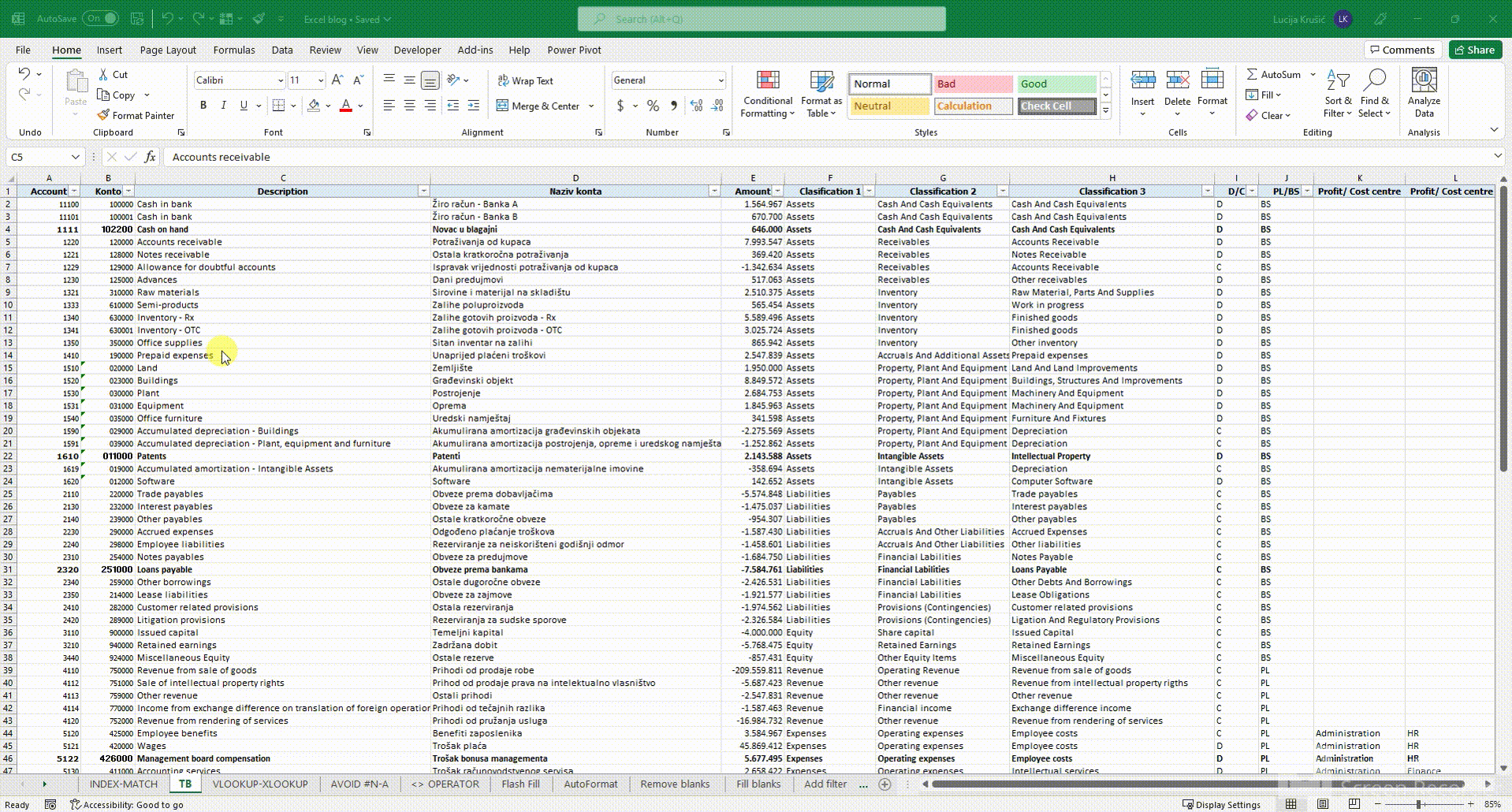
When working in Excel, have in mind that one thing can usually be done in a few different ways. You just have to pick the one that suits you the most. Knowing how to reference information in another tab or workbook is crucial for everybody in the finance sector. I started with INDEX, moved to VLOOKUP, and gratefully accepted XLOOKUP when it showed up.
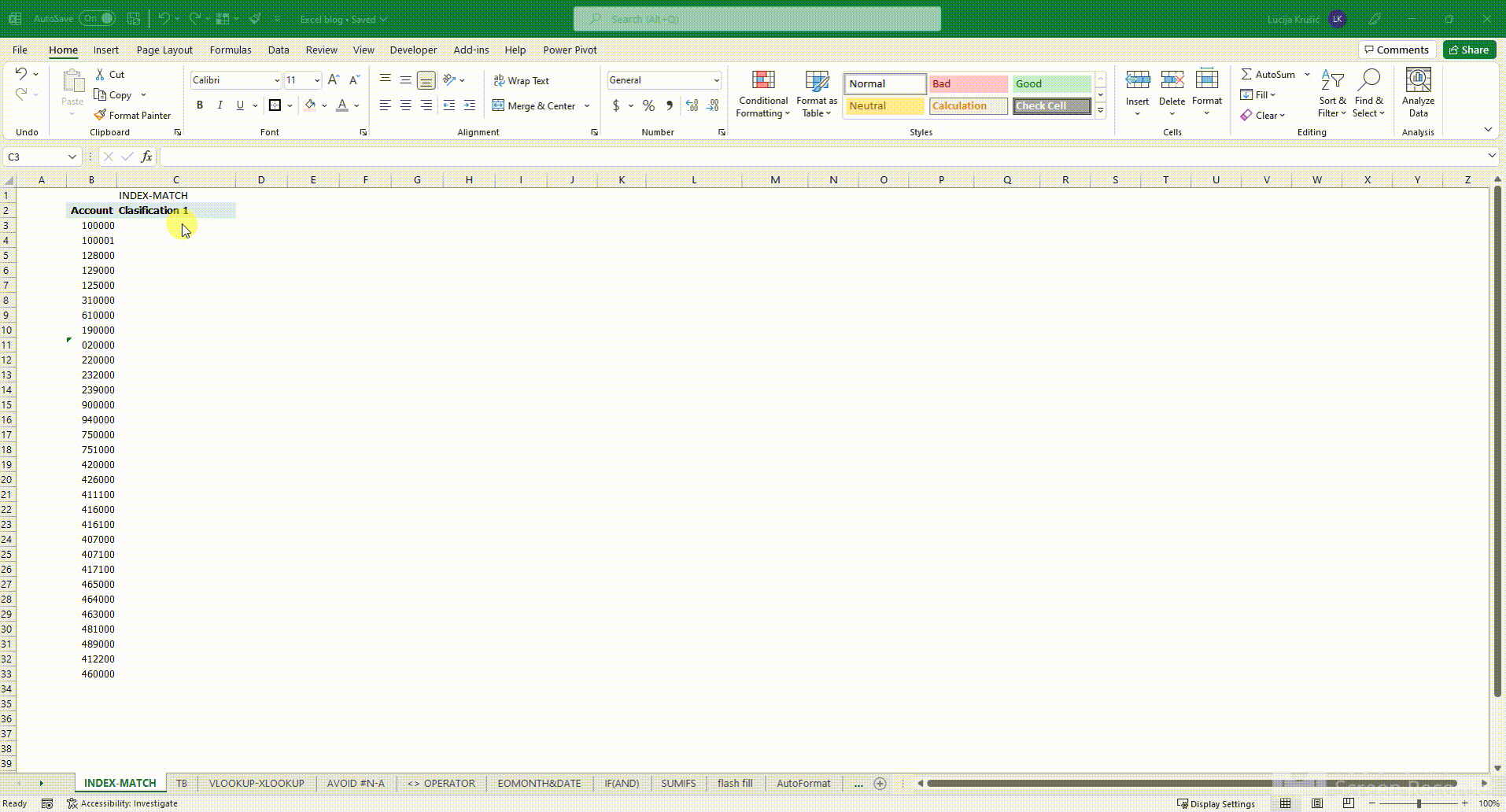
INDEX/MATCH
For most people, it is better to use INDEX/ MATCH than VLOOKUP and XLOOKUP. For the things I needed to get done daily, though, VLOOKUP and XLOOKUP were much simpler and faster methods. Nevertheless, it's good to know how to combine these two formulas for complex referencing.
ROW and COLUMN numbers from the INDEX formula are replaced with the MATCH function.
*Hint: The MATCH function searches for a specified item in a range of cells, and then returns the relative position of that item in the range. If you need to use it on its own, try also the improved XMATCH function.
Here's how to combine these two formulas to reference something:
VLOOKUP
The main problem with VLOOKUP is that it's static and it's always referencing the left-most column. This can create a lot of manual adjustments to the tables you are trying to combine. It is also a bit harder/slower to write the formula than to use XLOOKUP because you have to select the whole table and the number of the column you want to get as a result.

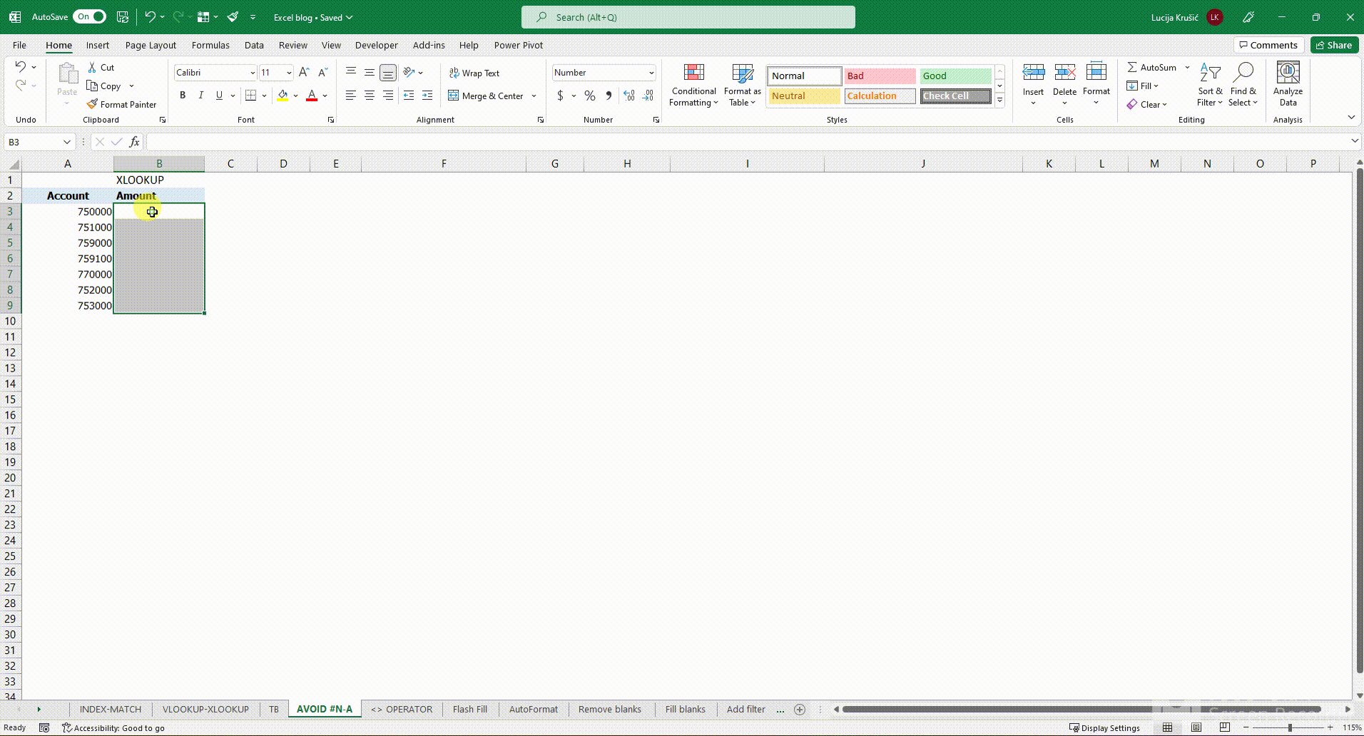
XLOOKUP
I prefer XLOOKUP to VLOOKUP because you don't have to select the entire table for it to work, just the columns you use for the formula. This also makes it dynamic when there are changes in the original table. XLOOKUP also has a built-in feature for errors (if not found).
The problem with this formula is that it's available only with newer Excel versions... I am sorry for some of you that still do not have it. ☹
Usually, when I get the data I need, if I don't expect any changes, I paste formulas as values, mostly because I am using XLOOKUP for data from two different Excels, and that can get a bit messy.

2. IF (AND)
IF is one of Excel's most popular functions and is used for logical comparisons. This pretty simple function can solve rather complex arguments when combined with AND function.
In the IF function, you basically have two results between a value and your expectation. One if the result is true, and one if it is false. You, the user, are the one that manages what these results are going to be.
So, you can just combine multiple IF formulas with AND function.

3. SUMIF(s) and other IF(s)
IF is often combined with other functions, and SUMIF is probably the most used one. SUMIF is used to sum the values in a range that meets your specified criteria. You can use it for either the exact criteria (like summing all the values above XY), or you can apply the criteria to a range and sum the corresponding values in a different range.
Logically, if you need to meet more than one criterion, you are going to use SUMIF(s). You can also combine IF with other functions like COUNT and AVERAGE.
*Hint: you can either write the criteria in the formula or reference the cell that has it. I used both in the example below:

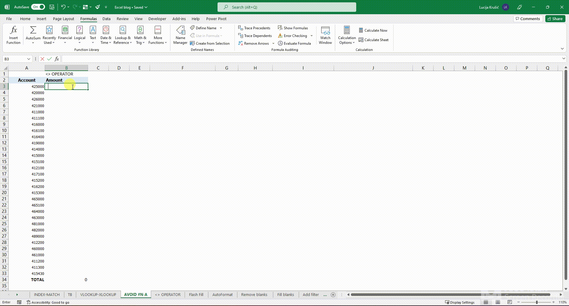
4. #N/A and how to avoid them (IFERROR and <> operator)
The best way not to have these as a result of a formula is to use the IFERROR function before the formula. Usually, I want a 0 value if the rest of the data are numbers or a blank space if it’s a string/text.
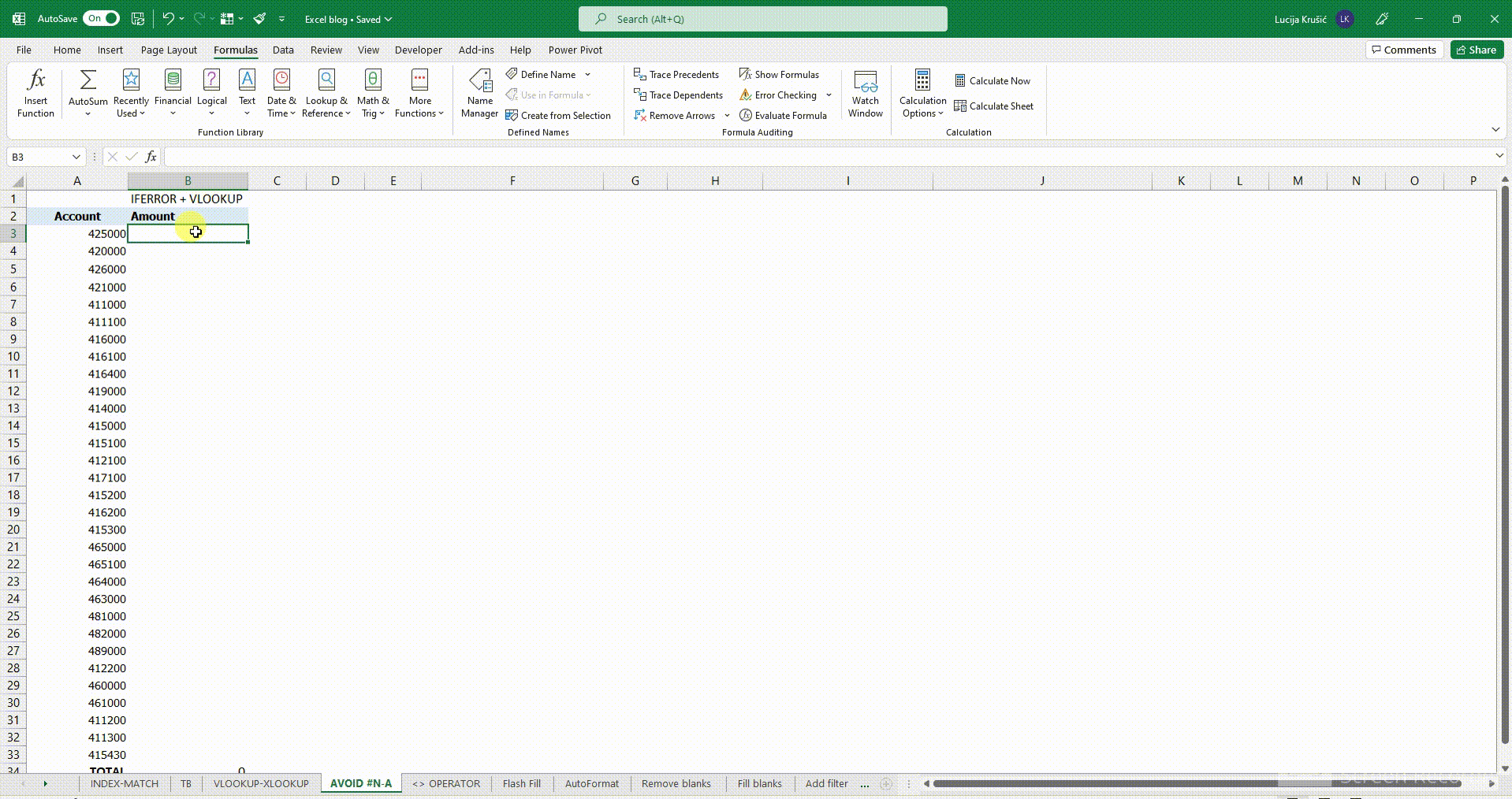
HINT: Remember that XLOOKUP has a built-in IFERROR (if not found) feature
If you want to sum the columns in which some cells have #N/A, and you forgot to use the IFERROR function and don’t want to change the formula again, it is best to use the <> operator. The <> operator in Excel represents not equal to. I think that it is self-explanatory, and it can be used for a lot of formulas.
In this case, it is combined with the SUMIF formula.
5. FILTER BY BOLD TEXT or similar (advanced FIND AND REPLACE)
This one is not a formula, but one of my favorite hacks.
As you all probably know, Excel supports filtering only by color or numbers. So, if you want to filter by bold text, for example, you have to get a little bit creative.
The way I am doing it when I get raw exports from ERPs that I have to clean is with an advanced find and replace function.
In the Find part of the Format section, you can choose to use the format from a selected cell. For example, a cell with bold text in it. In the Replace section you can format the cell in the color of your choice and use it to filter by it later:
6. EOMONTH/ DATE
This one comes pretty handy when you need to (re)calculate amortization (or depreciation). Usually, companies start the amortization in the month after the activation date. You can use these two formulas to get that date.


If you think that your financial models are overgrowing spreadsheets, and you need a better financial modeling tool, Farseer might be for you:
- Financial modeling in Farseer is centralized, fast, and consistent.
- You won’t need to worry about errors and mistakes.
- Natural language formulas are intuitive, error-proof, and cannot be deleted by accident.
- Sharing and exporting your work is granulated - you can share only parts of your model relevant to your user
- Built-in hierarchy makes modeling transparent by default - Reorganize models by simply dragging and dropping entire spreadsheets to a specific location in the model

LEARN MORE ABOUT FARSEER HERE